Procedural Content Generation

Introduction, Motivation

With every new generation of games hardware, making games is becoming a larger undertaking. Early games in the console and home computer era quite often were designed and programmed by one person who was able to fulfill every position required. Compare this to current AAA games that require hundreds of team members including many artists responsible for creating the game world in all its details. On the other hand, many indie teams are small and have a very limited budget. This has led to a growing interest in the recent years in procedural content generation, an ever-growing collection of techniques for building game content in an efficient, (semi)-automatic way.

Some of the earliest examples of PCG are Rogue (that spawned the large field of “Rogue-likes”) and Elite. In Elite, the universe is spawned from a single seed value, allowing the exploration of a vast space at a time when this size would not have been possible otherwise. Rogue fascinated players by generating a new playing field every time the game was restarted.

Some of the advantages of using PCG are the following:

• Open Worlds: PCG is an optimal complement to “open world” games, in which players are left to roam freely. A prime example is Minecraft, which is very open for players and generates a world they can freely explore and manipulate.
• Replayability: If a game generates new content each time it is played, this increases the replayability, thereby also increasing the shelf life and sales generated by the game.
• Small size: Instead of saving each asset of the game in binary form, a content generator can re-create the content from a small representation such as a random seed. In this way, games can be tuned to be as small as possible, for example to decrease download times in the case of apps downloaded via cellular connections. Many demos such as .kkrieger use PCG to reach incredibly small code sizes.
• Many details: PCG can be used to create a very detailed world, without requiring a designer to place every single detail. One example are object scattering algorithms which can place a large number of props (e.g. trees, rocks, …) in the world.
• Reduced costs: Quite often, small teams employ PCG as a means to build content they would otherwise not be able to produce with their budget. For a PCG algorithm, it might be sufficient to produce a small number of input elements to allow the generation of a much larger and more varied output of assets.
• Game concepts relying on PCG: Some games have concepts that would be impossible without PCG. “Endless platformers” are such a concept. In such a game, the player can continue playing virtually forever, with the world being constantly created.
• Adaptation to player preferences: PCG algorithms can be designed to adapt to the play style and preferences of players. If the PCG algorithm detects that a player would like to play the game in a certain way (e.g. if they want more enemies), it can adapt the generation parameters and generate content that fits the player’s preferences.
• Unique experiences: Probably one of the most intriguing situations in PCG is when a generator generates an output that even the designers and programmers had not foreseen. Since every now generated content is potentially unique, players can find an almost endless variation. This is the reason why Minecraft players exchange interesting seed values that spawn worlds with intriguing properties.

Main principles

Two main principles are often put in relation while creating a PCG algorithm: Structure and randomness.

Structure

Most PCG algorithms are able to create one instance of a class of objects. For example, a generator for houses will probably be able to create many different houses, which still share some basic structural elements. There will only be a certain number of different roof styles that the algorithm generates.

An important concept on which many PCG techniques are built is that we, as PCG users, do not care about concrete instances of objects, but rather about the class of objects. The realization of the PCG technique is finding what makes out the class of objects, and finding ways to create instances of this class.

As an example, a generator for 3D models of houses might follow a strategy of randomly creating a blueprint of the house, extruding the walls of the house and placing a roof on this house. It then can generate a number of houses with similar style. However, if the generator is only programmed to create one type of roof, the system will never create other types of roofs.

Randomness

Randomness is not a necessary feature of PCG, but it is often found in PCG algorithms. If the PCG algorithm generates a new instance each time it is run, this can create unforeseen structures and increase replayability. Randomness can also mean that the process of creation is governed by stochastic processes which still can be repeated. One of the alluring features of Minecraft is that each time you start it, you get a completely new world and start in a different environment. However, if you want to exchange a specific world with another player, you want to have the same world. In this case, you can exchange the seed value of the PCG algorithm’s random number generator to allow the other player to re-create the exact same world.

In cases where specific art is created for a game with PCG, it is often advantageous to have an exact and specified result. For example, the demo .kkrieger realizes a very small file size by creating the textures at the start of the game. Since an artist has fine-tuned the look of the game, having a random influence on textures might have a negative impact on the overall look and coherency of the demo. Therefore, PCG is here only realized as a mechanism for minimizing the file size and not for creating new content based on random input.

Further principles

Further principes of PCG are the following (this list is taken from the PCG book, see www.pcgbook.com)

Online versus offline

Online generation refers to generators that are called for example each time the game is run. This means that PCG is done on the end user’s system. Offline refers to tools such as PCG algorithms that are added in level design or other tools that designers or artists use. The PCG is run during the creation of the game, and the resulting assets are shipped with the game and can therefore not be changed. However, they can also be fine-tuned.

Necessary versus optional

If PCG is necessary, the game would not work without PCG. This means that the procedural generation is at the core of the game or there would simply be no game if the PCG was not run. Optional PCG, on the other hand, simply adds things like background objects or ambient sounds to the game, which do not influence the game experience that much.

Degree and dimensions of control

PCG algorithms differ in the amount of control and the way they give control to users. Some algorithms will be essentially a black box, while others have many parameters to fine-tune how they work. Often, different users are also exposed to different levels of control. The creators of Minecraft have a large amount of control over the way the game handles PCG, while normal players only have control over the random seed and a few select parameters that the algorithm uses.

Generic versus adaptive

Generic PCG approaches do not react to the actions of players and adjust the resulting content to them; adaptive PCG approaches do so. This could for example mean that players in a platforming game who evade many enemies and rather try to run through the levels as fast as possible get more challenging levels concerning jumps and fewer enemies, to better cater to their preferred play style. This also means that the PCG will probably have to be online to be able to react to the players’ actions.

Stochastic versus deterministic

Stochastic PCG approaches use randomness in the way the generate content. On the other hand, deterministic approaches wind up with the same result each time they are run. As noted above, also a deterministic approach can have randomness as a part of their operation. Stochastic PCG can add variation and replayability. Deterministic PCG can allow designers and artists to fine-tune the result of PCG. One aspect can also be related to making sure that nothing offensive is created by the PCG algorithm. For example, the designers of the original Elite game checked the names of all galaxies that their algorithm created, and in this way found that it would generate a galaxy called “Arse”, which was not intended by them.

Constructive versus Generate-and-test

Constructive PCG algorithms are carried out once and then the created content is used. Generate-and-test approaches use the PCG result and then test it for certain properties. This is related to genetic approaches in PCG, where genetic algorithms are used to search for an optimal PCG result.

Automatic generation versus mixed authorship

In mixed authorship, a player or designer takes the result of a PCG algorithm, refines it in some way or adds contraints that the PCG algorithm should take into consideration. After this, the PCG algorithm is run again, refining the existing content or adding new content that is based on the old. In this way, the designer and the PCG algorithm take turns in creating content.

Teleological vs. Ontogenetic

Broadly, PCG algorithms can also be divided into teleological and ontogenetic variants. Ontogenetic (ontos - being and geneia - mode of production) refers to PCG algorithms that are based on the analysis of the result of the PCG algorithm and finding ways (by whatever means) to reach these goals. For example, generating terrain heights by using a random noise function does not have much to do with the real processes which form real mountains, but the end result looks convincing enough for humans.

On the other hand, Teleological approaches (from telos - goal) are inspired by the real processes which result in the things depicted by the PCG algorithm. A teleological terrain generator might mimic the processes of tectonic movement to form rough mountains and the process of erosion for smoothing them. The end result will be more realistic and the approach might allow realistic animation of the stages that lead to the result, but will often also be less efficient than using the ontogenetic approach.

Toolbox

In the following, we look at some algorithms that are part of the “toolbox” of algorithms that are quite often used in PCG. This toolbox is not comprehensive, but instead intended as an introduction to the way PCG is often approached. It is interesting that some algorithms have several uses in PCG, as we will point out below. Further below, we will like at some algorithms and procedures in more detail.

Random Number Generators

We are not handling random number generators in this lecture, but they are often a central component of PCG. For our purposes, we just assume that we can call a function over and over and it will yield a new random number each time. Furthermore, we can set a seed value for the random number generator, and if we use the same seed value at a later point, we will get the same results.

Regular Languages, Grammars, Automata

Since PCG algorithms often use structured processes to construct instances of a class of objects, grammars and automata are well suited for describing these processes. An example will be given below in the form of L-Systems, which are commonly used to generate vegetation such as trees or bushes.

Noise functions

Related to a random number generator, a noise function can give use random values that have certain shapes that we can influence. For example, Perlin noise as will be described below, will have the advantage of being continuous, so that when we construct for example a terrain mesh from the noise function, the mesh will not be jagged, but instead will have a smooth shape.

Graph algorithms

Often, PCG algorithms generate intermediate steps that are then turned into the final asset for the game. For example, a map for a game could be described using a graph structure. This graph could then be transformed according to the rules a designer has specified to match the game for which it is created.

Genetic algorithms, heuristics

The approach of genetic alogrithms as often used for PCG algoritms. A set of specifications define what makes a good procedurally generated asset. For example, a heuristic might evaluate the quality of a level that is being generated. The genetic algorithm would then generate several levels, and only those would be evolved that indicate that they have potential. In this way, the algorithm searches the design space of all assets that can possibly be created with the chosen PCG algorithm.

Texture Generation

One interesting area of PCG algorithms is texture generation. We will be using it to exemplify the approach of PCG and also how PCG algorithms can be combined and controlled.

The goal of texture generation is the generation of a texture, which can include, apart from the diffuse texture we use to look up colors, also other associated textures such as the normal, displacement or specular maps. The output can also not only be used for being mapped to an object. Generated textures can also work well as height maps from which terrain can be generated.

We will be combining different approaches in texture generation as nodes in a network. Each node has one or more inputs (such as textures that it uses or parameter values) and one or more outputs (such as the resulting texture or parameters to use in further steps of the calculation).

Three types of nodes will be used:

• Basic generators: These nodes are placed in the network to get content into the network. They generate regular or random patterns which can be used in subsequent steps. This category also includes image inputs, since it might in some cases be easier to add a hand-created image or photo instead of trying to create it.
• Filters: These nodes work on the output of other nodes and transform it. This can mean that colors of the original images are changed, that the images are blurred, enhanced or in some other way modified.
• Combinations: These nodes bring different images together. We can imagine that we start with different basic generators and lead the outputs of them through the network of nodes. To create on image from the inputs, we need to combine the inputs.

In the following, we give some examples for generators, filters and combiners.

Basic Generators

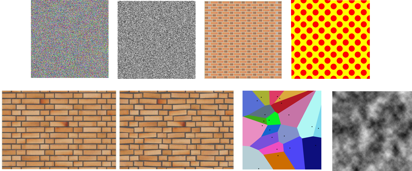
• Pixel Noise: The simplest type of noise is pixel noise, which chooses for each pixel in the generated texture a random color. This type of noise does not have any rules which relate the pixels with each other. A simple rule that can be added is to have only monochromatic noise, meaning that all random pixels have the same color, only different shades of this color. One obvious color choice that can be used is the range of grays.
• Solid Color: This generator just fills the whole texture with a specified RGBA color.
• Grid: This generator fills the texture with a grid. Parameters are the color of the grid lines, their thickness and the space separating them.
• Further patterns: Any kind of pattern, such as dots, circles, boxes, ornaments or other patterns can be used.
• Jittered patterns: A very rigid pattern can give the procedural nature of a texture away very fast. Instead, the pattern can be “jittered”, i.e. a small amount of randomness can be added. Instead of creating a brick wall in which all bricks are exactly the same size and orientation, small changes can be added.
• Random noise: As noted above, noise functions have advantages over purely random textures. We will be showing how to create Perlin Noise further below.

Filters

We already encountered filters in a previous lecture: Bilinear filtering used the values of 4 pixels (2 in each axis) to determine the value of one pixel in the resized/resampled image. This is one example of a filter kernel.

This kernel determines how many and which pixels we have to sample and how to combine them. The resulting pixel is the combination of the input pixels as determined by the kernel. For applying the filter, we move over all pixels of the source image and evaluate the kernel when it is centered on this pixel. Therefore, the kernel dimensions should be uneven, so we have a clear center pixel.

An example kernel is given below. The kernel shown is is not normalized: Its entries do not add up to 1. It can be normalized by dividing all entries by the sum of all entries before normalization. If the kernel is normalized, it will not change the brightness of the input image.

The kernel shown here is a blur filter. It will blur the image by taking an average of all the surrounding pixels and choosing this as the new pixel value. See the slides for more kernels with different effects.

During the execution of a filter, we have to decide how we handle the edges of the image. Just as in texture sampling, different options are available. We can just ignore border pixels, we can extend the border value, the image can be repeated, or we can use a constant color for sampling outside the image.

Gaussian Blur

One very common blur filter is the Gaussian blur. This filter uses the Gauss distribution in 2D as the values in the kernel. The values of the kernel are calculated by setting the expected value, mu, to zero. This way, the bell curve is centered at the origin. The standard deviation sigma determines the shape of the bell curve. A high deviation shapes the bell wider and less high.

The Gaussian blur is an instance of a separable filter. This means that instead of using the NxN 2D kernel, we can use a 1D filter kernel and first blur in one direction and then in another. In this way, the resulting image will be the same as if the 2D kernel had been used. However, we have less multiplications and additions to carry out, which makes this variant faster.

For larger kernel sizes, it can be advantageous to carry out the filtering in the frequency domain. Mathematically speaking, what we are doing while filtering is a convolution. In the frequency domain, the convolution becomes a multiplication, which is faster to compute. To transform the image into the frequency domain, we could for example use the Fast Fourier Transform algorithm.

Combinations

The last way in which textures can be generated is by combining two previously generated textures. This is done in a way very similar to the way in which we carried out alpha blending. Depending on how we combine which alpha values and which color values, different ways of combining results. Terms can be combined with all mathematical operations (e.g. multiply, add, subtract, …) to get different results.

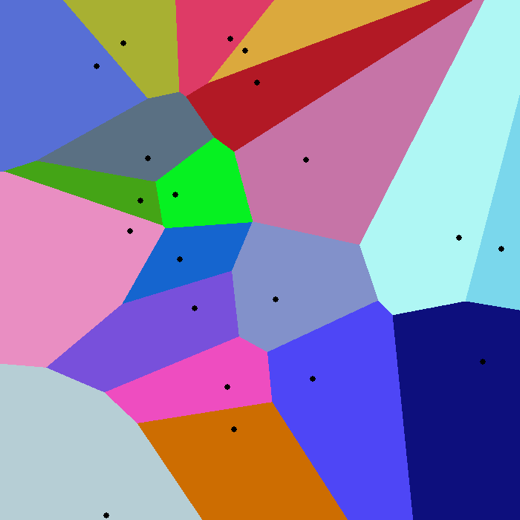
Voronoi Diagrams

Voronoi Diagrams are a commonly used tool in PCG algorithms, not only in texture generation, as we will see below.

A Voronoi diagram of a set S of points is a map that defines regions around each point in S. The region for point s is defined in such a way that no point in the region is closer to another point than it is to point s. To get an intuitive understanding of Voronoi regions, it is probably useful to have a look at some example configurations.

A Voronoi diagram of a set with only one point in S is made up of one region that encompasses the whole area of the diagram. In the case of two points, we see that we bisect our area, with the border between the points being a line. For a regular grid, we can get different configurations.

Computing the Voronoi Diagram

A Voronoi diagram can for example be computed by using Fortune’s algorithm. We will not go into all details of the algorithm, but we will look at the way in which the algorithm works in general.

Fortune’s algorithm is an example of a sweep line algorithm. The basic idea of such algorithms is to keep track of an area that is safe to compute. All the objects on one side of the sweep line have already been computed, while those on the other side still need to be handled.

For a Voronoi diagram, this would mean that we would keep track of the Voronoi diagram of all points on one side of the sweep line. For the other points, we would add them to the Voronoi diagram in the order in which the sweep line crossed over them.

The problem of such an approach is that points that are infront of a straight sweep line could still influence the Voronoi diagram on the other side of the sweep line. To handle this aspect, Fortune introduced a second “line” that follows the sweep line.

This line is defined in such a way that it is the boundary between the points that have already been computed and the line. For a single point, this line is a parable. All points that are on one side of the parable are closer to this single point, all other points are closer to the line.

When the sweep line moves, the parable “grows” as the distance to the line grows. When a second parable is added by the addition of a point, the parables intersect. To form the “beach line”, as the second sweeping line is called, we intersect them and take only the segments that are closest to the line. The shape of this intersection will usually look somewhat like a beach or waves that are moving towards a beach. For all sites the beach line has passed over, the Voronoi diagram can be computed safely.

Two kinds of events can be found in the algorithm. The first one is a “point event”. This event takes place when a new parable is added due to a point being added.

The second kind of event controls the placement of edges and vertices of the Voronoi diagram. This event is referred to as a “circle event”.

We can observe that some parable sections will start collapsing as the sweep lines moves away. The points where the beach line changes direction, i.e. where a new segment starts, are referred to as breakpoints. We can see that these points have, at any moment in time, equal distance to the two points that define the parable segments. Therefore, the movement of the break points during the algorithm trace the edges of the Voronoi diagram - the lines which have equal distance to two points.

When a parable section disappears, the point where it disappears is the center of a circle that is equally distant to three points that define the three parable segments it is defined by, and also equidistant to the sweep line. Therefore, when a segment collapses at a point, we find a vertex of the Voronoi diagram. When the sween and beach line have passed over all points, we have the Voronoi Diagram for the input set of points.

Examples of Voronoi diagrams in games

The developers of “Sir, you are being hunted” have described in detail how they created the look of their game. The game is played in a pseudo English countryside, which is defined by patches of land which are separated by hedges. Each cell in a Voronoi diagram is defined as such a patch. Hedges are placed on the edges, and for each cell, the algorithm determines what is placed inside (e.g. trees, fields, …). For more information, there is a talk available on youtube: https://www.youtube.com/watch?v=GYYuhuarTA0.

Another example is the “MapGen” demo by Amit P., which can be found at http://www-cs-students.stanford.edu/~amitp/game-programming/polygon-map-generation/demo.html

Noise

Noise is one of the most basic tools for procedural content generation. We will focus on the appplication of noise to texture generation, but noise can be used in many systems in games to control content creation or behaviour.

Perlin Noise

Pixel noise has, for many application areas, very disadvantageous properties. The pixels have no relation to each others. If you interpret the texture as a two-dimensional function, it has (usually) at no point any smoothness, meaning that the derivatives are jumping all over the place. Also, the resulting texture will often not look realistic as nature rarely has complete randomness. In the real world, objects will usually cluster together to a certain extent and changes will be gradual instead of sharp. No surface on earth is every 100% planar or completely random.

To address this challenge, noise functions have been proposed. Probably the best-known noise function is “Perlin noise”, named after computer graphics researcher Ken Perlin.

Perlin noise is a gradient noise. This means that we specify the gradient, or slope, of a function at certain points and interpolate in between these points. For a 1D Perlin noise function, we would specify a random slope at each integer point. At the same time, we define the function value to be 0 at these points. The interpolation is then done by taking the influence of the two closest integer points (e.g. 3 and 2 for 2.8) and calculate a value from those. We could just use the distance to the integer point as a weight factor for linear interpolation, however, Perlin suggests to use the fade function f(t) = 6t^5 � 15t^4 + 10t^3.

In practice, the gradients will not be random each time, but instead be drawn from a set of gradients in a repeatable way. For this purpose, the algorithm uses a permutation table of the first n integer (e.g. 256) which is used to draw the gradient.

The result is a function that is continuous in 1D and is zero at all integer positions. Due to its formulation, values are between -1 and 1. To display them as grayscale, we will usually transform them to be between 0 and 1. Furthermore, the function is usually normalized, meaning that the input value is mapped to the range 0 to 1.

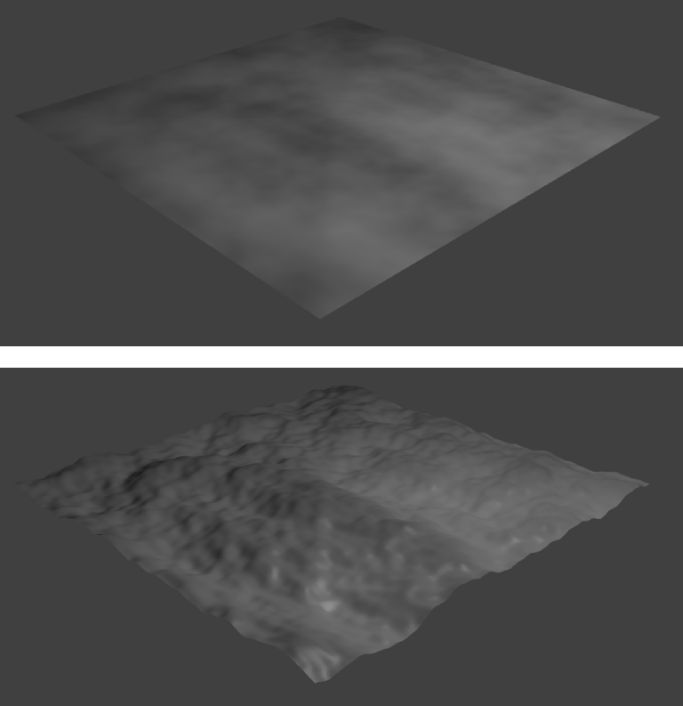
In many uses of Perlin noise, several instances of Perlin noise are combined with each other. We will be using two terms in this case: frequency and amplitude. Frequency is changed by changing the input value, amplitude by changing the output value. If the frequency is doubled each time, we speak of octaves as in music (if we double the frequency of a tone, we get the tone one octave higher). Usually, the amplitude is halved, meaning that the values will be in a smaller range. This combination can be interpreted well if we imagine that we create a terrain from the values. The low frequency and high amplitude octaves give us the basic shape of the terrain, with mountains and valleys. Higher frequencies and lower amplitudes give us small detail such as small crevices or hills.

In 2D, Perlin noise is defined by 2D gradient points at the integer grid points. The interpolation happens very similarly. To get the influence of each adjoining integer point, we take the dot product of the vector to the point in question from the sample point with the gradient at this point. The interpolation is then again done with the fade function, first in one axis (e.g. the x-axis) and then in the second axis (e.g. y).

Simplex noise

For several reasons, Perlin has later published Simplex noise, which is an advancement of his previous noise functions. We will not be going into simplex noise here. Advantages are that Simplex Noise scales better in higher dimensions and can give more levels of continuity.

L-Systems

L-Systems, named after the researcher Prucinciewyz Lindenmayer, are formal grammars that are often used for the generation of trees. Since the early days of computer graphics, very convincing vegetation has been created.

L-Systems are grammars that define symbols that are replaced during the execution of the creation algorithm. During each step, as many symbols as possible are transformed. This can be likened to the growth processes of plants and trees. Pieces of branch will grow larger and longer. New sprouts will form, which will later be “transformed” into new boughs or leaves.

To account for the nondeterministic look of real vegetation, L-Systems can include probabilites which govern how symbols are replaced. This leads to differently looking trees being generated from the same start symbols.

The resulting strings are usually transformed to 3D models using a turtle algorithm. The turtle follows the string’s instructions and places 3D object elements such as branches or leaves as encoded in the string. This can also be used to save space in the game: The trees could be transmitted to the players’ machines as strings which are then turned into tree models only when needed.