Artificial Intelligence
Introduction, Motivation
Many types of games would simply not be possible without Artifical Intelligence (AI); others would be lacking severely. Some of the main motivations for AI are the following:
- No need for other players: If, for whatever reason (for example, the game is not played intensively enough to find others playing at the same time, players want to train for themselves or there is not network connection) there are no other players to play with, the game can add AIs to play the other players. Also, in team-based games, teams can be filled up with AIs for example to balance the number of players.
- PVE (Player vs. Environment): In some multiplayer games, the players are not pitted against each other but against the game itself or the “environment”, i.e. computer-controlled characters. In this case, the AI can take control of the enemies in the environment.
- Realistic world: AIs are not only employed for controlling humanoid characters, but can also control other entities in the world. Examples are animals such as schools of fishes or flocks of birds that populate the world and make it more believable.
- Challenge: AI can also provide a challenge to players that a a human might not be able to provide.
- Testing: For testing a (single or multiplayer) game, AI can come in very handy. AIs can handle tasks that human testers might not be willing to do (such as test all collision bodies in the game by running into them). In multiplayer games, an AI can allow a single developer to test a game without getting other developers to play with him or her.
It is important to consider that artifical intelligence techniques are not only employed to simulate characters. For example, the prinicples of AI can also be applied for other components of games where intelligent choices have to be made. An AI technique could suggest edits to a level designer for example.
History
Certainly one of the fields that garnered a lot of attention in AI early were algorithms for playing the game of chess. Some of the first AIs for chess actually were not artificial: shady operators put small persons into chess “machines”; they would give out a move in response to a human player’s move. This became known as a “turk”, which is also the reason for Amazon’s crowdsourcing platform being called “mechanical turk”.
Later on, chess computers started actually working. However, in computer game AI, the techniques used in board game AI are often not so important. The main difference is that the state space of a regular computer game is often multitudes larger than that of a board game. For example, players in a 3D game can walk almost anywhere, carry out actions in any sequence, leading to a virtually infinite state space.
The beginnings of computer game AI can be traced back to the first examples of the genre. As the games were still in their infancy, so where the AI techniques. For example, the hard-wired AI of Computer Space (1971) determined in which sector of the screen a player was and fired a shot in this sector. Later on, simple Pong AIs stood in when no human opponent was there and controlled the paddle by keeping it on the same height as the ball.
Pac Man’s (1980) AI played, as the game itself, an important role in making AI visible. The ghost characters in Pong all have slightly different behaviours. Even though they are very simple, players often reported that they felt like they were planning ahead and acting differently.
Later on, games emerged where the main premise of the game was to have AI at the core. The “Creatures” series of games, started in 1996, allowed players to teach AIs (simulating neural networks) new behaviours and breeding them to create new creatures.
Game AIs have grown from these humble beginnings. Today, almost all games feature artificial intelligences. The techniques necessary for games have grown to a point where it makes sense to encapsulate them into libraries that are sold separately from game engines.
Academic AI vs Game AI
In artificial intelligence, there are two large strands that differ in their approach. One strand is concerned with really modeling the processes behind intelligence. The second one does not care about the way in which a decision comes about, but rather in the plausibility of the decision.
In game AI, like in game graphics, the ruling paradigm is often to reach a sufficiently good solution with the least computational costs. As Jim Blinn put it for the area of graphics, “All it takes is for the rendered image to look right.”. Therefore, also game AI most often uses techniques that might not result in ultra realistic results, but in results that “feel right”.
For example, many AIs could easily overpower a player. If FPS AIs were allowed to shoot perfectly, they would often annihilate human players. Similarly, brawlers such as “God of War” often only allow only a subset of the many enemies on the screen to enter melee fighting, otherwise, the player would become swamped. As the perception system of human players is overwhelmed by the graphics and sound involved, they will usually not recognize this situation as artificial.
Movement
The first layer of AI we will be looking at is movement of AI characters. This basic requirement is true of most AIs, and can only be skipped if there is no graphical representation of movement.
The basic idea of this layer is to turn the character into a certain direction and giving it a speed respectively acceleration. The result, over the course of several frames, results in a movement. Often, the animation system (for playing the correct animation) and the physics system (to tell if obstacles have been hit and to handle the acceleration of the character) are involved in this step.
Two basic variants exist on the movement layer: Kinematic and dynamic approaches. Kinematic approaches update the velocity (direction and speed) of a character immediately. The resulting movement can be blocky, instantly changing the direction the character is facing and it’s trajectory. The more believable system is dynamic, where the output of a steering algorithm is not a velocity, but instead an acceleration. The character will be accelerated into the given direction until a maximal speed is reached.
The algorithms described in the following can be applied to different dimensions: 2D games, 2.5D or 3D. Often, even games rendered in 3D can be broken down to 2D, for example a real-time strategy came with maps that have no overhangs can use 2D to handle movement. For games such as FPS games where characters can change the level they are on by climbing or jumping, we can get a away with 2.5D (3D position + 2D orientation). Only if the game inherently requires 3D movement (eg. a flight simulator) we need to use full 3D.
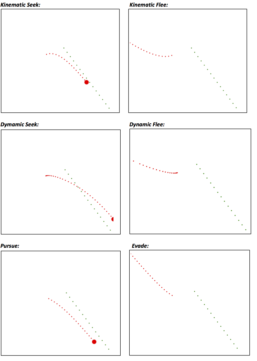
Seek and Flee (kinematic)
The first two movement algorithms we look at are Seek and Flee. In the following, A is the character we are controlling, and B the target (a position or another character).
For Seek, we take the vector from our position to the target (B - A), normalize it and multiply it by the maximal speed of the AI character. This makes our character move directly towards the goal with full speed. For Flee, the output of Seek is reversed by multiplying it by -1, moving the character away as fast as possible.
Arrive (kinematic)
Seek has the property that it can overshoot and then get into a loop, never fully reaching its target. The idea of Arrive is to define a radius around the target character. Outside the radius, we calculate the speed we would need to reach the target in a fixed amount of speed. This speed (clipped to the max speed) is given as the output of the algorithm. We can see that as we get closer to the radius around the target, we will slow down, settling in on the position of the target.
Wander (kinematic)
For characters that randomly walk about, we can use Wander. Here, the new velocity is chosen randomly, giving preference to new directions that do not change the orientation too much.
Seek and Flee (dynamic)
For making Seek and Flee dynamic, we again find the normal vector pointing from A to B. Now, we multiply it with the max acceleration of A. This leads to A accelerating straight towards B. For Flee, the output is again reversed.
Arrive (dynamic)
Similar to kinematic Arrive, the dynamic variant should slow down when it gets closer to the target. A target velocity that gets closer as the goal is reached is computed, and an acceleration is output that will lead to the desired velocity.
Other behaviours
Align is used to choose the same orientation as the target.
Velocity matching will match the velocity of a target.
Delegated behaviours
Delegated behaviours build upon the primitive behaviours we have looked at so far.
Pursue and Evade
For Pursue and Evade, we take our full speed into account and compute how long we would take to reach the target if we travelled at full speed. Then, we compute the hypothetical position of the target if it moved forward with its current speed and use this new position as a target for a Steer (pursue) or Evade (flee).
This way, we can intercept characters that are moving, instead of chasing them.
Wander
For delegated Wandering, we delegate to a dynamic seek operation. The input for the seek is given by choosing a random position infront of us inside a circle of specified size. Since the acceleration that is output will not change the orientation instantly, the wandering behaviour is smoothed.
Path following
When we follow a path (e.g. computed by a pathfinding algorithm), we can use a Seek behaviour to guide us towards the next way point.
Separation
Separation describes that we want to stay away from other characters. To achieve this, we calculate the strength with which the other characters around us push us away, and move away from them accordingly.
Collision Avoidance
A collision avoidance behaviour will strive to avoid imminent collisions. A simple variant could just check for characters infront of us. A more complex variant could check if the paths of the two characters will really intersect, and only act if this is the case.
Obstacle and Wall Avoidance
Similar to collision avoidance with other characters, an obstacle/wall avoidance behaviour will try to keep characters clear of walls. The basic mechanism for this is to cast rays (one or more) infront of the character.
This method can lead to problems, for example at corners in the level. If the AI faces the corner, one ray should tell it to turn left. In the next frame, the next ray, which now intersects closer to the AI, tells it to turn right, leading into an endless loop that keeps the AI stuck. This problem is not easy to solve and could be solved by special corner-handling code or changing the size of the fan of rays when such a loop is detected.
Combining steering behaviours
A game character will use several behaviours. For example, it chases a target, at the same time it avoids obstacles as well as other characters. There are different possibilities to implement this.
One possibility is to use blending, optionally with weights for each output. One example for this approach is Flocking as described by Craig Reynolds. This technique is used often to simulate natural phenomena consisting of several entities interacting, such as school of fish or flocks of birds. Each “boid” (entity) has an individual steering behaviour. It is combined of three behaviours that are blended:
- Separation (move away from close-by neighbours)
- Move in the same way as the flock (match avg. velocity and orientation)
- Cohesion (steer towards center of the flock)
In practice, such a blending system can reach a deadlock in the form of an equilibrium, where the resulting blended output is zero. For example, if the chased target is straight ahead, but a character to be avoided is standing still right infront of it, the two blended outputs could cancel each other out. This equlibrium can be instable, such as the one just described (since a slight change in the configuration could break it), but can also be stable, if even larger changes do not break the deadlock.
Another option is to define priorities for the current situation. If the system detects that collision avoidance is the most important, it can value this system higher. However, in a stable equilibrium, this could still not break the deadlock: if the fallback behaviour is stopped before the equilibrium is left, the default behaviour/weights can steer the character back into the equilibrium.
One possibility is to break up the independence of the basic steering behaviours. For example if a Seek and wall avoidance behaviour can communicate, they can find a more optimal solution for the character than the blending of the two.
Pathfinding
The next level is to tell an AI where to move, using global data in the form of the level or world data. This path is then followed using the movement systems.
In the majority of cases, pathfinding is done on a graph in which the basic connectivity between two nodes indicate that the two points in the world they represent can be reached. An assigned weight of an edge indicates how “hard” it is to move between the two. If edges are directed, the situation can arrive that an AI can traverse it only in one direction (e.g. jumping down a ledge).
When we query the pathfinding system, we need to find nodes for world positions. This process is called quantization. The reverse, mapping nodes to world positions, is called localization.
Almost all game AI systems use (a variant) of the A* algorithm. We will not handle the algorithm details here.
Once a way through the network has been found, it is desirable to smooth it so the artificial nature of the game characters is not as easily seen. This can be achieved by several methods, for example by checking if sub-paths of the path can be skipped by analyzing the space between the nodes in question.
Graph Generation Methods
Designer-specified
Some systems require a level designer to define the graph structure themselves. This leads to more work, but can result in high-quality graphs due to the knowledge of the designer. Also, these graphs need to be manually adapted when the level changes.
Points of visiblity based
An automatic algorithm for the generation of the graph is based on the points of visibility of the level. Here, we start with all corners in the world. We move the possible node positions away from the corners so that a character can fit on the node and not be stuck in the corner.
In the next step, the visibility between the nodes is checked, resulting in a very dense network of nodes. To be usable, the network has to be pruned to bring the number of nodes and edges down to a reasonable level.
Navigation Mesh
In another automatic method, the mesh of the floor defined by the artists and level designers, is used as the basis. A node is placed on each triangle of the floor. Then, the connectivity between the nodes is checked as before and, if necessary, the graph is pruned to bring it down to usable size. For example, the pathfinding mechanism in Unity uses this system.
Hierarchical pathfinding
If a characters is asked to navigate over a large map, it could for several reasons be unreasonable to compute a detailed graph for the whole way. For one, the character could be intercepted along the way, the path could change (e.g. the player issues a new movement command), or the terrain might change. In this case, it is more reasonable to find a broad path to the target and only compute detailed paths for the area just infront of the AI.
This can be done by defining clusters of nodes and computing the paths between these clusters. When finding a path, we find out in which cluster we and the target are, and compute a path consisting of clusters. Then, we follow this path, only calling the detailed pathfinding when we enter a new cluster.
Movement planning
A specialized way of pathfinding can be used when the character have a limited set of animations that need to be played for a certain movement speed. In this case, we could use an A* variant that can handle infinite graphs, and consider at each node the possible animations that we could play from this node. In this way, a sequence of moves is found that lead from one position to another.
Decision Making
In order to know where to move to, an AI needs to decide on what to do. Besides the movement system, this can involve other systems as well, such as playing certain animations or triggering other actions in the game world.
Several methods for decision making are common in games. The end result is usually a state in which the AI is. This state is often realized as a function that is periodically called and in which the AI carries out the actions associated with the state. For example, a “chase player” state might turn the AI towards the player and accelerate it in that direction.
One thing to prevent for all decision making methods is oscillation between states. For example, when an AI is close to a distance at which it will switch states, it can make sense to add hysteresis, so that it can not be stuck between the two states. Furthermore, when random decisions are made, it is important to make sure that the AI will not switch to another state whenever its update function is called.
Decision trees
A decision tree has the states of the AI as the leaves and decisions as the intermediate nodes. As the tree is traversed, conditions are checked, such as “is distance to player < x”. The tree is usually designed based on the game design or can be learned using machine learning.
A good rule of thumb for efficiency is to place computation-heavy decisions lower in the tree, so they are called less frequently.
State machines
The most common mechanism for decision making is games are finite state machines. Here, states can be freely connected with other states. A transition to another state is triggered when the conditions for it are met.
The state machine will usually be created by a designer, and specialized graphical tools assist with creating it.
An important evolution in state machines are hierarchical state machines. Here, several state machines are used to describe the state of an AI, and the active state can switch from one to the other. One example where this can help with keeping the state machines usable is when an AI should have some kind of “alarm” state that overrides all other states. Without hierarchical state machines, this “alarm” state would have to be reachable from all other states. If a second FSM is used, we can instead define the alarm state in terms of this second state machine.
Behaviour trees
Behaviour trees at first look similar to decision trees. Differences are that instead of states, behaviour trees manage tasks at their leaves. Furthermore, the intermediate nodes are not only decisions, but can also indicate sequences of tasks, repetitions of tasks or random choices.
Utility-based AI
Behaviour trees can become very complicated and hard to manage. A paradigm that operates without any of the pre-defined state transitions of decision trees, FSMs or behaviour trees is Utility-based AI.
Utility refers to the current benefit an action can bring the AI in the given context. If an AI has no ammunition, reloading has no utility value. If it wants to shoot, the magazine is empty and it has ammunition, the utility of reloading is high.
In a utility-based reasoner for game AI, we usually use the following terms:
- Option: One of the things the AI can possibly do
- Task: The concrete action that is associated with an option
- Consideration: A test that maps the current game context to a utility value
A consideration is implemented as a re-usable test. Many considerations can be re-used in different contexts. For example, in the case of deciding whether to choose the option “flee” or “attack”, the health of the AI would be a consideration that is re-used for evaluating both options. The differences between different contexts are usually exposed to AI designers as curves that map the value of the consideration to a weight for the utility-based reasoner.
To choose an option to execute, utility-based AI uses a weight-based random choice. Each option is weighted by using the output of its consideration as the weight. Then, a weighted random choice is made. If option a is weighted with weigth 10 and option b with weight 1, this means that in 10 out of 11 cases, option a will be chosen. This indicates that option a is considered better than option b in this context.
This leaves the question of how to deal with extreme differences in weights and the associated “stupidity” if the low-weighted option is chosen. For example, if a is weighted at 0.01 and b at 10, this indicates that option a is very bad compared to b and would probably look unintelligent to a player if it was chosen. But, since we are using random numbers, it might just be chosen.
There are two counter-measures for this in utility-based AI:
- Cutoffs: We can immediately eleminate any options with weight = 0, since they will never be chosen. Furthermore, we can find the highest weight and cut off all options with a weight that is lower than x% of this heighest weight, or eleminate the lower quartile etc.
Ranks: Ranks are used to give importance to options beyond weight. While choosing a new option, we gather all ranks and find the highest one. Then, only those options with the highest rank are considered. This means that they are prioritized above all others. The rank is also found as the output of a consideration by mapping the value to a rank instead of a weight.
In this way, utility-based AI has no explicit state transitions. Instead, the AI always chooses the best option for the current situation. The design work is then to fine-tune the weight and rank-curves of all options to create a believable AI.
Fuzzy logic
Fuzzy logic is sometimes used in game AI. It is well suited for problems where decisions are not clear-cut but vague instead. For example, how much health of a character leads to it being “injured”? Fuzzy logic does not deal with such absolute attributes or set memberships. Instead, an object such as the AI has a set membership with an associated value between 0 and 1. So, a character might be a member of the “injured” set with a degree of membership of 0.7, which is more injured than a character with a value of 0.3.
“Fuzzyfication” then refers to turning a piece of game data into a fuzzy degree of membership, and “defuzzyfication” to the reverse process.
For fuzzy logic, the equivalents of the usual Boolean logic operators are defined in terms of equations on the associated degrees of membership, using combinations of min, max and subtraction operators. For example, “NOT A” is equal to 1 - a, and “A AND B” is equal to min(a, b), where a and b define the degrees of membership of A and B.
Based on these operators, we can define rules of inflection to find degrees of membership for new sets. For example in a driving game, if A defines the proximity to a corner and B the velocity of the car, then we might want to have a degree of membership for C, indicating that we should brake. The associated formula then is c = min(a, b).
If we have several formulas of this type (i.e. several rules which give different values for c), then we compute each rule individually and then take the minimum over all results.
Goal-oriented behaviour
Many game characters can be seen as entities that want to fulfill a set of goals (motives/”insistence”). For example, the Sims do not want to be hungry, be happy, … To reach these goals, characters have a set of actions. These actions typically depend on the game state (for example, if the character has no money, it can not buy food). They change the game state, for example decreasing hunger at the expense of money.
An AI can make decisions based on the goals it has and the available actions. The most simple way to choose an action is to choose the current optimum and not look ahead at the future. This will, however, not lead to longer strategies, meaning that the AI might not reach a global optimum. For example, it might be better to stay hungry for a while and then getting good food instead of snacking all the time.
Systems can add a value for the overall utility to the results of an action, indicating that some actions have a long-term positive or negative effect. Similarly, the time required for actions can be added, if timing is of the essence. However, these methods still do not look ahead more than one step, and therefore will not behave with a plan.
This can be achieved with goal-oriented action planning (GOAP), where instead of a single action, a sequence of actions is examined, and the state of the hypothetical future is taken into account. Such a system can be implemented with a variant of A* that can handle graphs with unknown or infinite size. However, even such a system might be unable to find a global optimum: if we look ahead 10 moves, but the optimal solution involves 10 “bad” steps and one final step which turns the whole situation around, we would not find it.
Blackboard architectures
Blackboard architectures are ways in which AI components can communicate with each other. Similar to a regular blackboard, a set of data is written to it, and others can read from it or change the data that is there. One advantage is that cohesion between components is reduced: new components can be added without explicitly adding code for handling the existing components. Furthermore, a decision making method can be built from such an architecture: each component gives an estimation upon being polled how well it can handle the current situation. Then, the component with the highest estimation gets control over the character.
Tactical and strategical AI
One level further up from decision making, systems for tactical and strategical AI are concerned with providing global information to AIs or with synchronizing the actions of several AIs.
An example are waypoint tactics, where waypoints for AIs are not only checked for being reachable, but also for their tactical value, such as whether there is cover at the waypoint. AIs which are planning an action can use this information in their decision making process.
Similarly, a tactical AI can analyze the game map and give an estimation of values such as the level of control of a player over a certain region, the danger associated with a region or other similar values. Such maps can be learned, for example by keeping track of where units have been destroyed (“frag maps”), or can be derived from the game state. The latter can be done for example by plotting on a map all the positions of units, and then adding values to adjacent cells/pixels based on the distance. This kind of map can also be reached by applying a blur filter.
Execution management
AI tasks have to be executed along with the other tasks of the game engine. For movement and decision making, the AI should regularly be polled. Furthermore, some tasks are created depending on the game state, such as a pathfinding operation for a character.
For each AI task, a frequency (how often should it be called?) and a phase can be defined. The phase defines the offset of the periodic call to a later frame. Using a good phasing, several tasks can be spread out over several frames instead of always slowing down every N’th frame.
Several methods for building a good scheduler exist. One method is “Wright’s method”, where we simulate ahead the next frames and count the number of tasks that will be run in each frame. Then, the frame with the lowest number of tasks is found. If all tasks before have been added in this fashion, it is propable that this frame is a good candidate to add the task.
Interruptible tasks and anytime algorithms
Since AI tasks often do not need to give an answer or result in something visible each frame (as compared to many graphical tasks), we can use algorithms that can be interrupted. For example, A* can typically be interrupted and continue at a later point. In this way, the pathfinding can be spread out over several frames.
A special class of algorithms in this regard are Anytime algorithms, which are built with the intent of being interruptible, and at the same time being able to quickly give an approximation of the optimal answer. The more time they are given, the better the solution will be. An anytime A* variant might be able to produce a valid path very quickly, and then improve the path when it is called again. Compare this to a regular A* implementation, which will not provide a valid path until the computation is complete, and then will not be able to improve it with more time.