Advanced Software Rendering
The previous forays into software rendering left three major graphical glitches unresolved.
Depth Buffer
More complex 3D objects have depth issues even when backface culling is used. All triangles would have to be sorted from back to front for correct rendering in all situations. Even worse, correct rendering of intersecting objects would require triangle sorting of all triangles of each group of intersecting objects. Realtime graphics nowadays use a depth buffer to solve all of those problems using an extremely simple algorithm.
foreach (pixel) {
	if (framebuffer[pixel.x, pixel.y].z < z) continue;
	framebuffer[pixel.x, pixel.y].rgb = rgb;
	framebuffer[pixel.x, pixel.y].z = z;
}
For every pixel the depth test checks for the smallest z value that was previously seen at that position. The depth test algorithm was avoided in earlier 3D games due to speed concerns but it works reasonably well when using dedicated hardware. However a depth buffer does not solve the depth sorting problem for partially transparent geometry. Modern games still today suffer from depth sorting problems when partially transparent objects are involved.
Perspective Correction
The combination of regularly interpolated texture coordinates and perspective projection creates skewed looking images and visible seems between triangles.
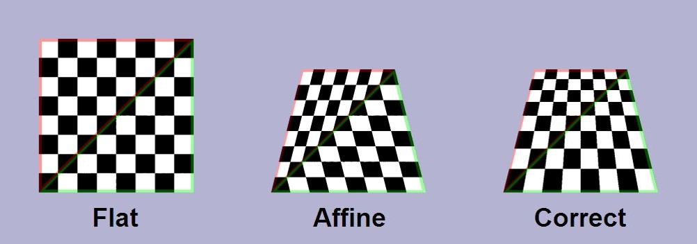
Regular linear interpolation is not sufficient in a perspective coordinate system. For a correct visual appearance, the coordinate divided by the depth value has to be interpolated to linearly shrink the texture according to the projected depth. The modified interpolation equation is
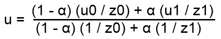
with α being the relative position (from 0 to 1) between the interpolated vertices.
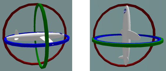
Rotations
The previous chapter showed how to calculate a camera view by calculating the rotations of the camera around the x, y and z-axis, the so called Euler angles, independently and one after another. Euler angle calculations depend on calculation order – rotating around x and then around y will yield different values than rotating around y first. Handling this correctly is not intuitive and when the calculation order is not chosen wisely one rotation axis can be rotated into one of the other two axis, which cancels out one degree of freedom. This situation is called the Gimbal Lock.
The rotation calculation around a single axis derived in the previous chapter by reevaluating coordinates in a new, rotated coordinate system.
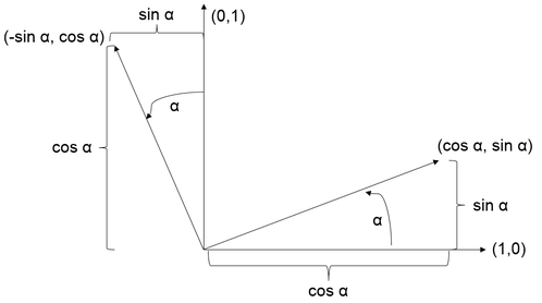
This resulted in the formula
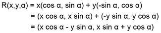
which is an example of matrix multiplication, typically written as
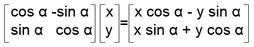
Rotation matrices
According to Euler’s rotation theorem any rotation or sequence of rotations of a rigid body or coordinate system about a fixed point is equivalent to a single rotation by a given angle θ about a fixed axis (called Euler axis) that runs through the fixed point. This basically defines a new coordinate system and can thus be integrated into a matrix which results in the formula
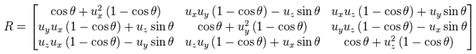
with u being the unit vector and Θ the rotation angle. This rotation matrix is a much bigger construct than three Euler angles, but it does not suffer from Gimbal Lock.
Transformation matrices
Matrix transformations can not only represent rotations but most kinds of affine transformations, which are all transforms which preserve straight lines like scaling, shearing and rotations. Matrices however have to be extended to also support translations.
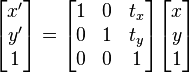
Adding an additional column to the transformation matrix and an additional line to the vector matrix makes it possible to represent translations. And adding an additional line to the transformation matrix makes it possible to support projective transformations. Creating a matrix like
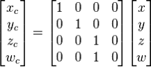
will divide every coordinate with its z component – the perspective division. Overall this results in the following matrix structure:
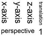
Matrices can be multiplied themselves with the results representing the combined transformations executed one after another. This makes using matrix multiplications a very useful technique for 3D graphics as large sequences of transformations can be precalculated and represented in a single 4x4 matrix.
The four component vectors shown in the translation and perspective transformations are a more general mathematical concept called homogenous coordinates which is used in projected coordinate systems. The four component vector is mapped to a 3D position by dividing x, y and z components with w – the fourth component. The other way round a homogenous coordinate is created by adding a w component of 1 to a 3D position. Direction vectors are represented by adding a w component of 0.
Quaternions
One important problem remains in handling rotations – rotations cannot be interpolated efficiently using Euler angles or rotation matrices. For that reason games widely adopted Quaternions for rotation calculations. A quaternion is a four dimensional imaginary number consisting of one real and three imaginary components which can represent a rotation around a vector u with an angle of Θ according to:

A point can be rotated using: rotated point = q * point * q^-1 Representing a quaternion using w as the real component and v as the vector of imaginary components multiplication is done according to: q1*q2 = (w1w2 - v1 · v2, v1 x v2 + w1v2 + w2v1)
Quaternion multiplication is not commutative aka q1 * q2 != q2 * q1. The inverse of a quaternion is: (w, -v) / (w² + x² + y² + z²)
The all-important quaternion rotation interpolation is implemented by
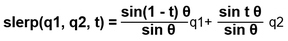
with
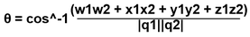
This is a proper spherical linear interpolation meaning that when the rotations are mapped to a sphere, the interpolation will find the shortest path between the two mapped points on the sphere.
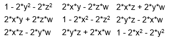
A quaternion can be represented as a matrix, making it practical to include quaternion calculations in a regular, matrix based transformation pipeline:
Lighting
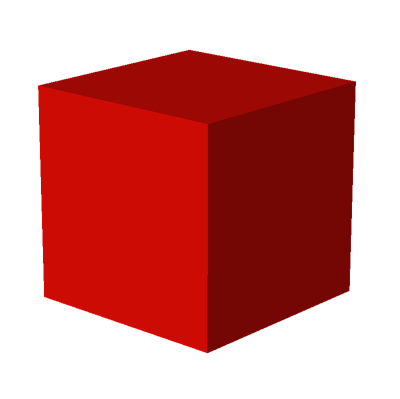
When all the basics of a 3D renderer are working the next obvious step is to add lighting. 3D meshes are mostly exported including normal data – the orientation of vertices which is then interpolated across the triangles to calculate the orientation for each pixel. Vertices are eventually duplicated before being imported into a 3D renderer to retain sharp edges where lighting information should not be interpolated. A popular example of that is a cube.
Calculating the dot product between the transformed normal and the direction to a light source yields a nice looking diffuse lighting.
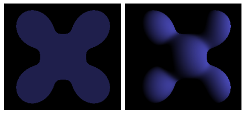
Light most mesh surface calculations local lighting can be calculated per pixel (interpolating the normal between vertices) or per vertex (directly using the normal and then interpolating the resulting colors between vertices). Per pixel calculations are generally more exact and nicer looking but also slower.